
How Does AlphaGo Work?
AlphaGo is a novel combination of deep neural networks, reinforcement learning, and Monte Carlo Tree Search (MCTS). It achieved state of the art performance at the time it was published and has defeated some of the strongest human players.
The algorithm mainly consists of three parts: policy network, value network, and MCTS search. On a high level, policy network is a simple CNN trained with supervised learning. Value network is policy network enhanced by reinforcement learning. MCTS search uses both policy and value network to perform look ahead search and return the next best move.
Policy Network
SL Policy Network
This is a simple 13-layer CNN trained on (board state $s$, next action $a$) pairs using supervised learning. Given a board state $s$, it predicts a probability $p_{\sigma} (a | s)$ at each board position that represents how likely an expert player would choose it as the next move.
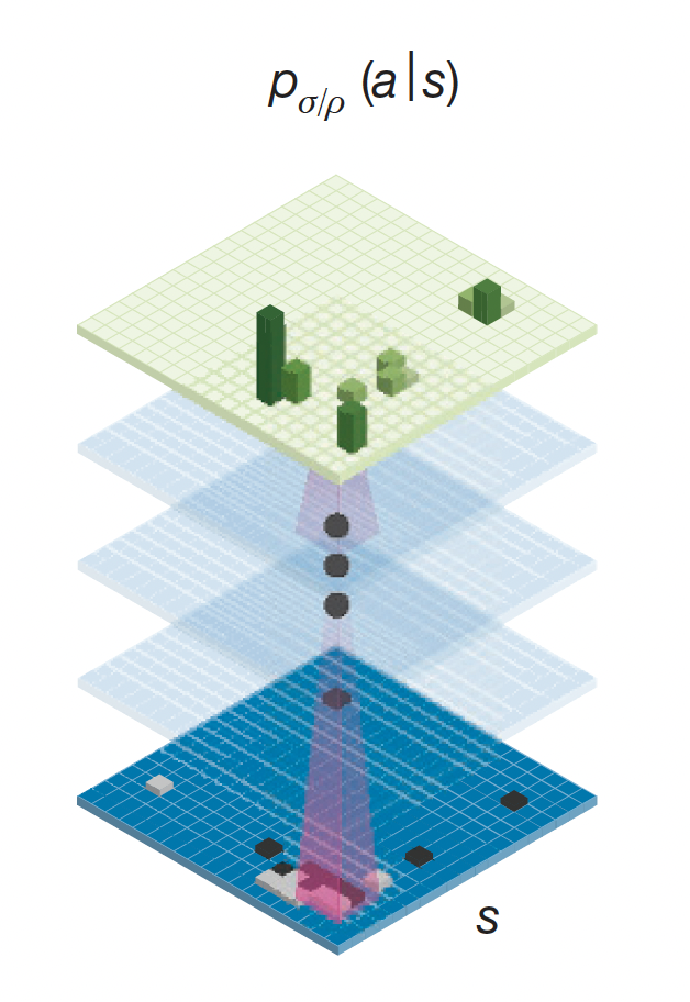
Fig.1. Illustration of policy network (Image Source: Mastering the game of Go with deep neural networks and tree search)
Fast Rollout Policy
$p_{\pi}(a | s)$ is a faster and less accurate version of the SL policy network. It has faster inference speed because there is no expensive convolution, only linear combination of features with softmax at the end to produce probability. The computation requires only dot products and softmax.
The features in the network are manually engineered to reflect common patterns in Go. My understanding is that this hand-crafting process replaces the need of convolution at the cost of accuracy. But that is okay, since the main purpose of this network is to have faster inference so that we can use it to perform more efficient rollouts during Monte Carlo Tree Search.
Enhancing Policy Network
One key idea in the AlphaGo algorithm is to improve the simple SL policy network through self-play. We use the network to play with a previous iteration of itself and update the weights to prefer selecting actions that are most likely to lead to a winning outcome. This is an application of the classic RL REINFORCE algorithm.
The self-play algorithm is as follows:
- Input: SL policy network $p_{\sigma^0} (a | s)$
- Output: RL policy network $p_{\rho} (a | s)$
- for $i = 1$ to $N$ do:
- $\sigma^i \leftarrow \sigma^{i-1}$
- Randomly select $j$ from $[0, i-1]$
- Run $p_{\sigma^i} (a | s)$ against $p_{\sigma^j} (a | s)$ to generate a complete game rollout $(s_0, a_0, s_1, a_1, …, s_T, a_T)$
- for $t = 0$ to $T$ do:
- If $(s_t, a_t)$ was played by the winner:
- $\quad$ $z_t \leftarrow 1$
- else:
- $\quad$ $z_t \leftarrow -1$
- $\sigma^i = \sigma^i + z_t \frac{\nabla \text{log} p_{\sigma^i} (a_t | s_t)}{\nabla \sigma^i}$
- $\rho \leftarrow \sigma^N $
- Return $p_{\rho} (a | s)$
Algorithm.1. Enhancing Policy Network Using Policy Gradient RL
The update rule updates the network weights to maximize probability of selecting actions that lead to a positive reward (i.e. winning the game).
Value Network
Unlike policy network, the purpose of value network is to predict the expected game outcome at a given state $s$ assuming both players use policy $p$. It is defined as:
\[V^p(s) = E[z_t | s_t = s, a_{t...T} \sim p]\]The network evaluates the expected game outcome at time step $t$ (a point in time during the game). At this time $t$, we have the board state $s$ and policy $p$. The network tells us that, if we keep sampling actions using this policy $p$ for the rest of this game, what would be the expected value of the game outcome.
Training
They train a network $V^w(s)$ with weights $w$ to approximate $V^p(s)$. The network is trained on state-outcome pairs $(s, z)$, using Stochastic Gradient Descent to minimize the MSE between predicted value and the true outcome $z$. The paper reports that overfitting occurs when some state-outcome pairs $(s, z)$ come from the same game. They create a new dataset of 30 million distinct positions $s$, each sampled from a separate game. The game was played between the strongest policy network and itself. Training on this new dataset solved the problem of overfitting.
Evaluation
The paper evaluates accuracy of the value network at different stages in a game (see green curve). They sample a bunch of state-outcome pairs $(s, z)$ from human expert games. Each of the position is at a different stage in a game (i.e. how many moves have been played in the given position). For each position $s$, they use a single forward pass of the value network $V^w(s)$ and compute the MSE between the prediction and ground truth outcome $z$. It can be seen from the graph that the value network prediction approaches the accuracy of Monte Carlo rollouts of trained policy, while being a lot more efficient. It only requires a single forward pass, while policy rollouts need to play out a game multiple times and take the average.
Another interesting observation is that the policy and value network can closely approximate outcomes of human games in later stage of a game. This makes sense because when a game is almost played out, it will be easier to predict the outcome, whereas there are many possibilities in early stages of a game.
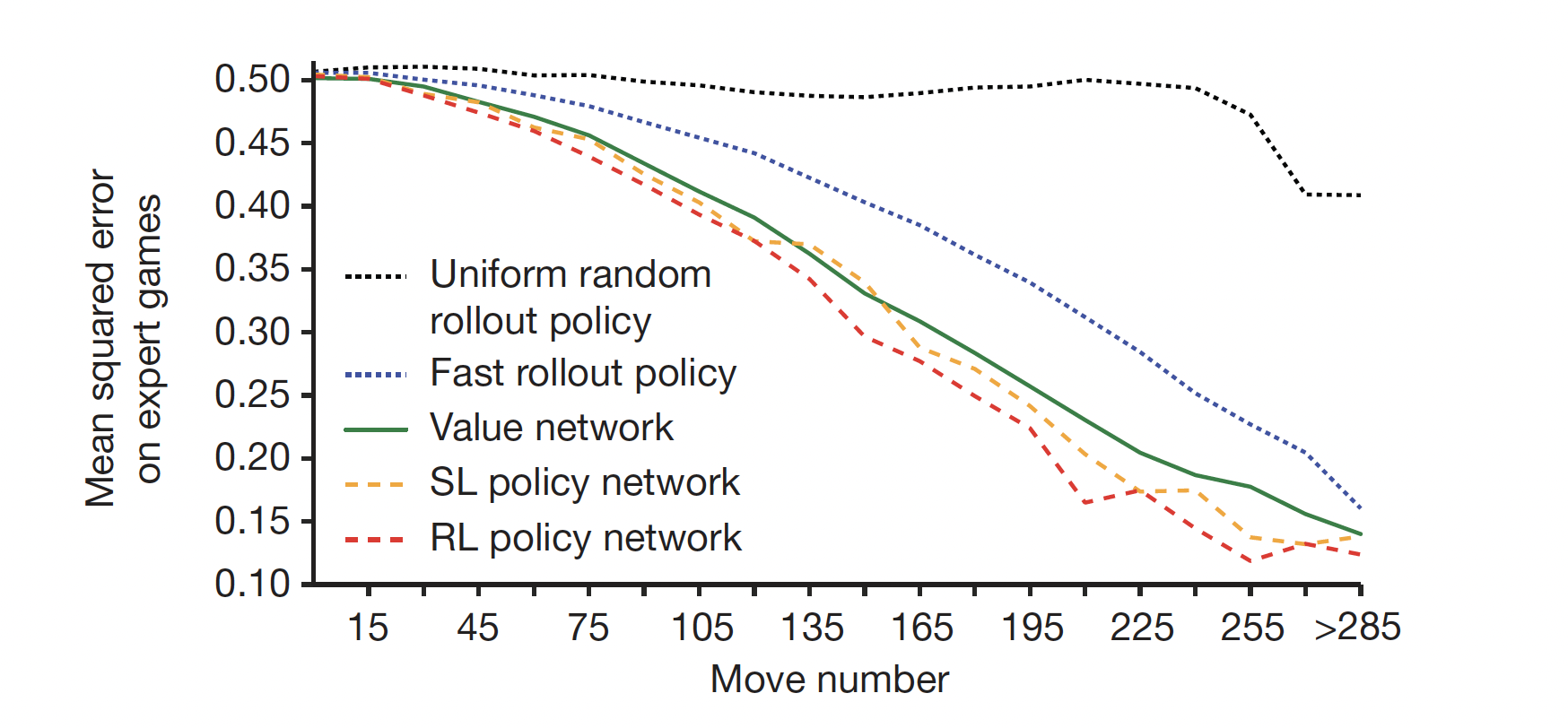
Fig.2. Comparison of evaluation accuracy between the value network and rollouts with different policies (Image Source: Mastering the game of Go with deep neural networks and tree search)
Monte Carlo Tree Search
AlphaGo uses MCTS to repeatedly simulating possible futures to get an idea of which move is most frequently selected from the current position. The move is selected in order to maximize reward plus the probability suggested by the policy network. The probability is divided by visit count in order to encourage exploration.
Algorithm
The following is the pseudocode for MCTS:
- Input:
- $\quad$ Current position $\hat{s}$
- $\quad$ Total number of simulations $N$
- $\quad$ Mixing parameter $\lambda$
- Output:
- $\quad$ Move $\hat{a}$
- for $i = 1$ to $N$ do:
- $s_0 \leftarrow \hat{s}$
- for $t = 0$ to $\infty$ do:
- If $s_t$ is a leaf node (i.e. has not been explored yet):
- Apply SL policy network and store $p_{\sigma} (a | s_t)$ for all legal moves $a \in A(s_t)$
- Estimate the expected outcome with value network $V_w(s_t)$
- Get outcome $z_t$ of a random rollout starting with position $s_t$ using fast rollout policy $p_{\pi}(a|s)$
- Combine the estimations using $\lambda$: $V(s_t) \leftarrow (1 - \lambda) V_w(s_t) + \lambda z_t$
- break (i.e. end of a simulation)
- else:
- for all legal moves $a \in A(s_t)$: $u(s_t, a) \leftarrow \frac{p_{\sigma} (a | s_t)}{1 + N(s_t, a)}$ where $N(s_t, a)$ is the number of times the edge has been traversed
- Select $a_t$ such that $a_t = \text{argmax}_{a \in A(s_t)} (Q(s_t, a) + u(s_t, a))$
- $a_t$ leads to the next state $s_{t+1}$
- Update visit count for all $(s, a)$: $N(s, a) = N(s, a) + 1(s, a, i)$ where $1(s, a, i) = 1$ if the edge $(s, a)$ was traversed in the simulation, $0$ otherwise
- Update value for all $(s, a)$: $Q(s, a) = \frac{1}{N(s, a)} \sum_{i=1}^{n} 1(s, a, i) V(s_t^i)$ where $n$ is the number of simulations run so far. $s_t^i$ is the leaf node encountered and explored in the $i$-th simulation.
- Return $\hat{a} = \text{argmax}_a N(\hat{s}, a)$
Algorithm.2. Monte Carlo Tree Search in AlphaGo
Visual Examples
For ease of understanding, below I drew a visual run-through of the first two simulations. We are currently facing position $s_0$ and need to make a move.
Simulation 1
We start at the current position $s_0$. Since it has not been explored yet, it is considered a leaf node. Therefore, we apply the SL policy network to get the prior probabilities for all legal moves.
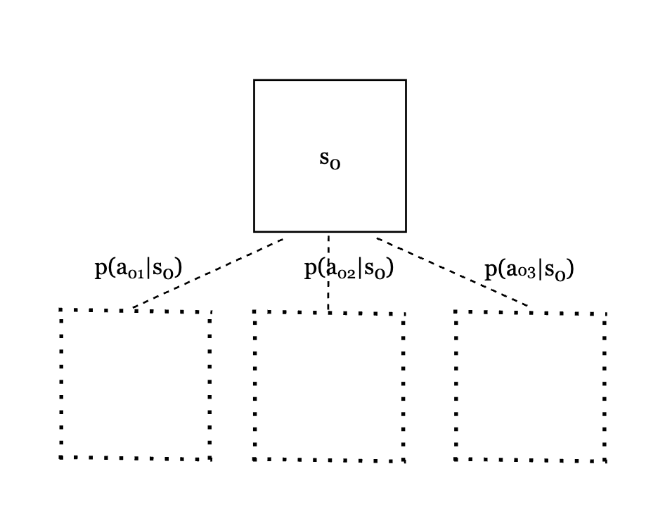
Fig.3. Prior probabilities for all legal moves
Then, we estimate the value at current position $s_0$. According to the algorithm, we need to do this by 1) applying the value network $V_w(s_0)$ and, 2) doing a fast rollout till end of game and recording the outcome $z_0$. The final value is combined by the mixing parameter $\lambda$. $V(s_0) = (1 - \lambda) V_w(s_0) + \lambda z_0$.
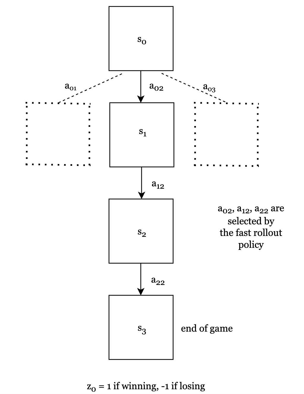
Fig.4. Fast rollout to end of game
We are now at the end of simulation 1 and need to update the visit count and value for all edges.
$N(s_0, a_{02}) = N(s_1, a_{12}) = N(s_2, a_{22}) = 1$ since they have been traversed. All other edges have count = 0.
$Q(s_0, a_{02}) = Q(s_1, a_{12}) = Q(s_2, a_{22}) = V(s_0)$. All other edges have value = 0 since they were not traversed.
Simulation 2
In this new simulation, we again start at the current position $s_0$. Since it has been explored in simulation 1, it is not a leaf node, and we need to select a move that maximizes value. In other words, from all legal moves, we need to choose move $a$ that maximizes $Q(s_0, a) + \frac{p (a | s_0)}{1 + N(s_0, a)}$
From simulation 1, we know that:
\[Q(s_0, a_{01}) + \frac{p (a_{01} | s_0)}{1 + N(s_0, a_{01})} = p (a_{01} | s_0)\] \[Q(s_0, a_{02}) + \frac{p (a_{02} | s_0)}{1 + N(s_0, a_{02})} = V(s_0) + \frac{p (a_{02} | s_0)}{2}\] \[Q(s_0, a_{03}) + \frac{p (a_{03} | s_0)}{1 + N(s_0, a_{03})} = p (a_{03} | s_0)\]So we will compare these three values and choose the maximum one and the corresponding move. $a_{02}$ is the move chosen in simulation 1. If it has a high prior probability and high value, then it will be chosen again. But the other two moves can be chosen if they have high prior probabilities.
No matter which move we choose, we will arrive at a leaf position that hasn’t been explored before. Then we can repeat the procedure in simulation 1 (i.e. getting the prior probabilities for all legal moves and estimating the value at that position).
Follow-Up Work: AlphaGo Zero
Dual-Head Neural Network
AlphaGo Zero uses a single network to predict both value and move probabilities given a position.
Monte Carlo Tree Search Improvements
In AlphaGo MCTS, the leaf node is expanded by 1) applying policy network to compute the probabilities of all legal moves and 2) using fast rollout to end of game + applying value network to get the value. In AlphaGo Zero MCTS, the leaf node is evaluated by the single network which gives both the value estimate and move probabilities.
Self Play Improvements
In AlphaGo self play training, the moves are selected by the policy network. We apply the network once to get the probability of all legal moves from current position, and choose the move with highest probability. In AlphaGo Zero, Monte Carlo Tree Search is used in self play. We execute MCTS at each time step and the moves are selected according to the search probabilities computed by MCTS.
No Use of Data From Human Games
The network training does not use human game data. Instead, it is trained on data generated from self-play. The network takes each raw position from self-play and produce a vector that represents the probability distribution over moves, and a scalar value that represents the value. The value label is the game outcomes of self-play rollout. The policy labels are the search probabilities produced from MCTS during each time step in self play.
References
[1] https://www.nature.com/articles/nature16961
[2] https://gibberblot.github.io/rl-notes/intro/foreword.html
[3] https://home.ttic.edu/~dmcallester/DeepClass18/16alpha/alphago.pdf
[4] https://dilithjay.com/blog/reinforce-a-quick-introduction-with-code
[5] Open source ELF OpenGo https://zhuanlan.zhihu.com/p/36353764
[6] https://www.nature.com/articles/nature24270